
How does the average rate of change between two points lead to the derivative at a single point?
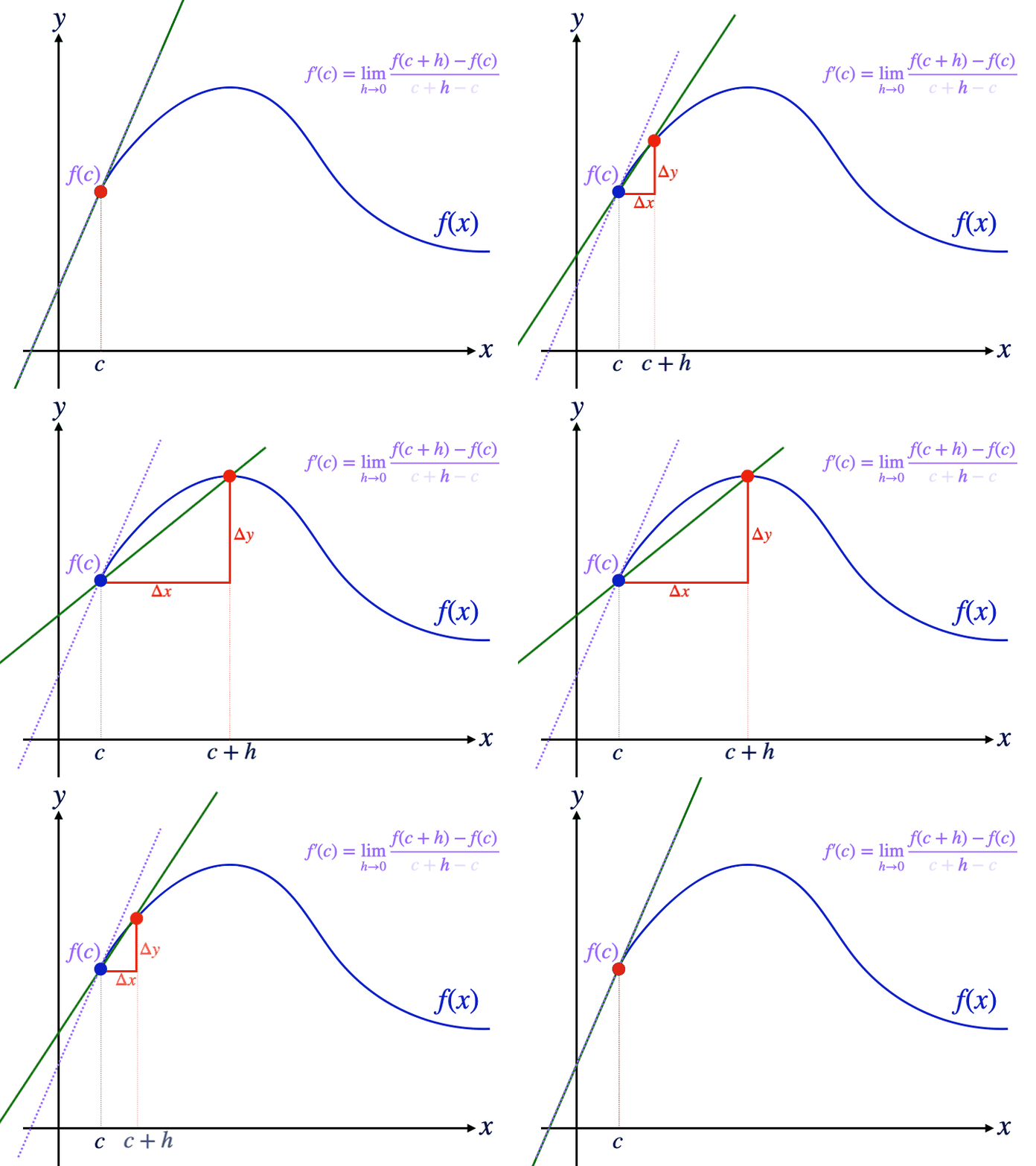
By the end of Unit 1, students can calculate limits and distinguish between average and instantaneous rates of change. Unit 2 brings those ideas together: as one point on a graph approaches another, students use a limit to calculate the instantaneous rate of change at a single point. Then they see how finding that rate at different inputs gives rise to a new function: the derivative.
The videos below are part of the complete AP Calculus AB/BC Animated Curriculum. As graphs, labels, and equations appear one step at a time, students can follow the reasoning that connects one idea to the next. The animation carries the visual sequence, leaving you free to watch your students, notice when something isn’t clicking, and respond in the moment.
As I get ready to start Unit 2 with my own students, I thought I’d share the first three animated lessons from this unit with our community. Start with both parts of Lesson 2.1 below. If you’d like to continue, click the button at the bottom of the page and I’ll send you Lessons 2.2 and 2.3—four more videos—along with guided notes for all three lessons.

At the heart of this lesson is a deceptively simple question:
How can something be changing if time itself isn’t?
It’s the kind of question that opens a door—a door into the true world of calculus.
In this first part of the lesson, I want students fully focused on the concepts. That’s why I provide all the notes in advance—so they can listen, absorb, and reflect without scrambling to write everything down. (You can download the guided notes PDF using the opt-in below the video.)
In Part 2, students take a more active role—applying what they’ve seen by working through problems and building their own intuition. For now, I invite you to press play and experience the lesson for yourself.
So go ahead—hit play, and let’s begin this journey into the heart of calculus.
💡 Want the matching guided notes and practice questions?
Download the PDF below to help your students follow along and reflect without distraction.
In Part 2 of this lesson, students shift from watching to doing. This video picks up where the first left off—with two clear, visual examples: one on instantaneous rate of change, and one on average rate of change—the kinds of questions they’ll see again and again.
I typically pause the video after each example, giving students time to solve, discuss, and build their intuition before revealing the animated solution.
Go ahead and press play to experience how this second part turns understanding into real problem-solving confidence.
The matching handout includes all the key ideas, plus space for students to solve the problems you just saw.
If you haven’t grabbed it yet, you can download it below.

I hope you enjoyed this animated introduction to calculus. This lesson is part of an animated AP Calculus AB/BC curriculum I’ve spent the past few years developing. The curriculum is now nearly complete, with the final Unit 10 lessons being added over the next few weeks.
I’d genuinely love to hear what you think. Feedback from fellow teachers has helped me refine and strengthen these lessons, so please don’t hesitate to reach out with any questions, suggestions, or thoughts about how the lesson worked with your students.
If you’d like the matching guided notes and practice questions, click the button below and enter your email. The PDF will be sent directly to your inbox.
I hope this lesson sparks curiosity, confidence, and clarity in your students.
Let’s make this the year calculus finally clicks.